DAX: Data Analysis Expression

Written by Julien Larcher – Technical Executive Associate

DAX for “Data Analysis Expression” is a programming language used in Microsoft Power BI to create columns, measures and calculated tables thanks to its numerous functions. In short, it’s a great way to enrich your data model. If I’ve lost you in the first line of this article by mentioning “programming language”, don’t worry, this article aims to demystify this language and hopefully provide you with some answers!

A few definitions

Calculated column

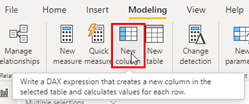
Add a column to a table. The data is added (calculated) only once, when the data is loaded (or updated). The calculated column will create a value for each row in the table. The column is physically stored in the data model, and therefore has an impact (sometimes significant) on file size.

Calculated measurement

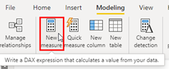
Add a measurement or indicator to a table. Data is calculated on demand. When you add it to a display, or when you change the value of a filter. Bear in mind that measurements are calculated according to the filters used in the report. Together, these filters represent the context. Unlike the column, the measurement takes up no space in the data model. Measurements primarily use processor resources to perform calculations.

Calculated table

Adding a table to our data model. In addition to retrieving tables from various data sources, you can also use DAX to create your own tables. The best example of this is the “calendar” table, which we can create entirely in DAX. There are specific DAX functions for creating tables (DISTINCT, VALUES, CALENDAR …).

DAX functions

make up the DAX language. These functions fall into different categories. There are aggregation functions (SUM, AVERAGE …), date and time functions (DATEDIFF, DATEVALUE …) and filter functions (ALL, ALLEXCEPT …). It is beyond the scope of this article to list all existing DAX functions – there are plenty of sites for that purpose.

Evaluation context

One of the most important concepts to understand if you want to master the DAX! The evaluation context represents the set of filters applied to the data. A DAX formula is always executed in a context, and there are two types of context:

Filter context (segment, page filter, visual filter, line or column)
Line context: this is the current line when an expression is evaluated (calculated column, for example).

We’re going to take a closer look at these different contexts to give you all the information you need to understand the keys to the DAX language!

The different contexts

Line context

There’s nothing like a good example to help you understand! The line context represents the current line when evaluating a formula.

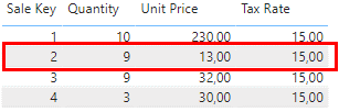
The table below represents a sales table containing a Sale Key, a quantity, a unit price and a tax.
If I want to add the sales amount associated with my sales line to this table, I need to create a calculated column.

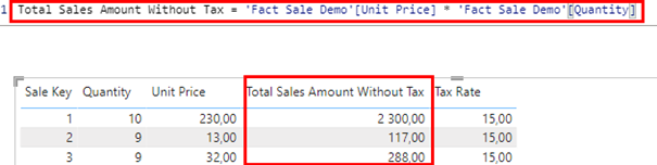
In this example, we can see that the calculation is performed for each row of our table. When creating a calculated column, DAX interprets the formula row by row by default.

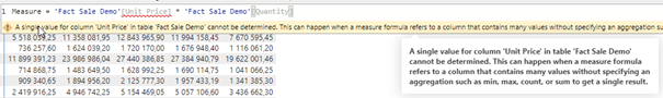
If we try this same formula, not in a column but in a measure, we’ll get an error message, because the measure doesn’t know, by default, the row context to use. We’ll need to use aggregation functions (SUM) or iteration functions like SUMX to properly define the row context the formula should use.

Filter context

Represents all the filters applied to the data BEFORE the DAX formula is evaluated.

In Power BI, the notion of filter represents any element allowing the segmentation of data, such as :

Segment (slicer)
Page filter, visual filter, etc. (filter banner)
Row and column in a matrix
Row in a table
X-axis and/or Y-axis in a chart

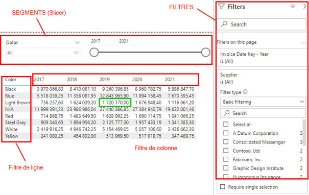
In the example above, the value 1,720,170.00 comes from our measurement:

Total Sales := SUM( ‘Fact Sale'[Total Including Tax] )

This measure is simply a sum of our sales amount. The fact that we have a different value in each cell comes precisely from our filter context. Here, the data is filtered on the color “Light Brown” and the year 2019.

By using the colors in the rows and the years in the columns, the matrix data is filtered and the result of our measurement is found at the intersection of the 2 elements.

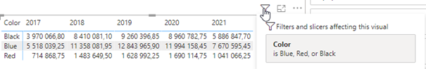
It’s true that with this multitude of filters, we can quickly get lost in our visual and no longer know which filters are being applied… but that’s without counting on Power BI’s help with the visual header, which offers a feature that lets you see which filters or segments are currently being applied to the visual.

The Calculate function

We won’t go into detail about all the DAX functions here, but one of them deserves our full attention: the Calculate function!

This function will be used to modify the execution context of a DAX formula.

Let’s go back to our example:

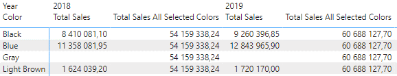
In this matrix we use 2 measures :

Total Sales = SUM ( ‘Fact Sale'[Total Including Tax] )

This measurement is calculated using the row and column filters in the matrix.

Total Sales All Selected Colors = CALCULATE( ‘Fact Sale'[Total Sales] ,

ALLSELECTED( ‘Dimension Stock Item'[Color] ) )

To this end, we modify the execution context using the CALCULATE and ALLSELECTED functions. In this way, we obtain the amount of sales for all colors combined, while maintaining the filter on the year. This can be used to create a ratio, for example, to obtain the weight of a particular article color in sales for a given year.

The key point here is that the CALCULATE function must be used whenever we wish to modify the execution context of a DAX formula.

Use the right relationships

Another DAX function deserves the spotlight: USERELATIONSHIP.

In a Power BI data model containing two tables, for example :

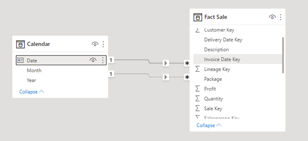
The classic case of a fact table containing several dates and a calendar table.

In this example we have two existing relationships between the FactSale fact table and the Calendar table, but only 1 relationship is active. This means that all analyses involving a notion of time will use the invoice date by default.

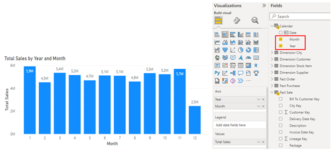
This graph shows the evolution of sales per month from the invoice date. We are using the calendar table and our Total Sales metric. By default, this measure will use the active relationship on the invoice date.

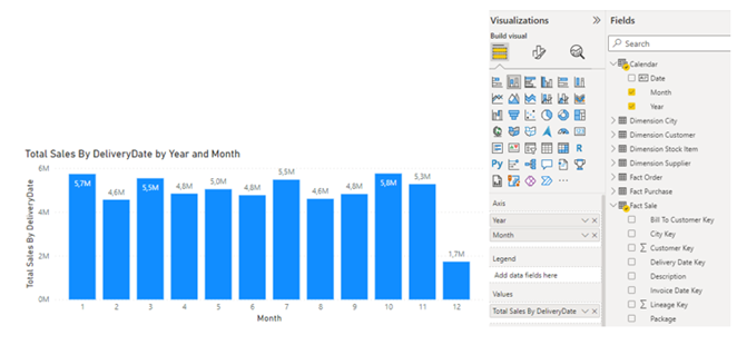
If our analysis is to focus on the delivery date and not the invoice date, we need to use the USERELATIONSHIP function to “activate” the correct relationship and thus tell Power BI to perform its calculation with the delivery date:

Total Sales By DeliveryDate = CALCULATE( ‘Fact Sale'[Total Sales] ,
USERELATIONSHIP( ‘Calendar'[Date],’Fact Sale'[Delivery Date Key] ) )

This is where we find our CALCULATE function, as we modify the context of the calculation with the USERELATIONSHIP function.