Written by Julien Oudille – ActinVision BI Consultant
In this article, discover how Power BI, via the DAX language, automatically uses clusters to group together combinations of values actually present in the data, a mechanism called auto-exist. This behavior, often overlooked, impacts filtering and measurement results, as only existing combinations are taken into account in calculations.
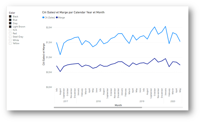
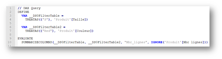
When creating a visual with Power BI, regardless of the storage mode or the complexity of the calculations, the underlying DAX query will always have the same structure, based on the use of the SUMMARIZECOLUMNS function. Take, for example, the chart below with a basic filter:
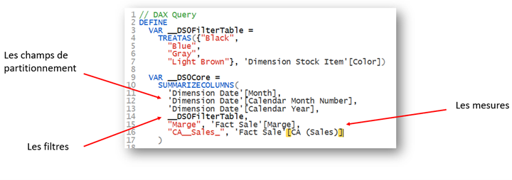
The DAX request sent and executed by the engine is as follows:
The SUMMARIZECOLUMNS function has 3 types of arguments: partitioning fields (visual axes), filters (table arguments) and measures. Discover how Power BI interprets a filter system consisting of several columns from the same table!
Case studies
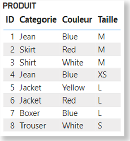
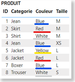
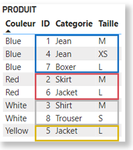
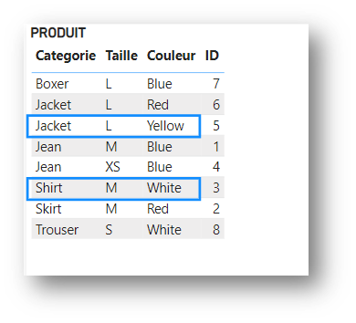
For the purposes of this demonstration, let’s consider the following PRODUCT table:
As soon as a table is called up in a DAX expression, Power BI creates what is known as a data cluster, corresponding to all the combinations of values actually present in the table.
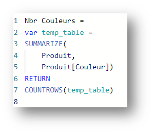
An example with the following measurement to calculate the number of distinct colors:
This query obviously returns the number 4.
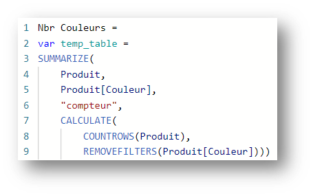
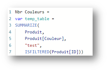
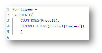
Let’s do a test by adding a counter for the number of rows in the global temp_table. Assuming that the only filter here is on the Product[Color] field, all we need to do is add the following expression:
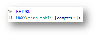
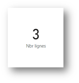
A MAX on this table should therefore always give us 8, but the following expression gives us the result 3 :
This is linked to the behavior of the SUMMARIZE function, which systematically introduces a data cluster depending on the table called up.
For each combination of values in the called columns, Power BI will also place filters on all the columns in the called table, according to the combinations of values present in the table.
The Product table, here grouped by Color, contains the following clusters for each color:
In other words, for the color Blue, Power BI introduces the following filter:
(ID = 1 and Categorie = “Jean” and Taille = “M“) OR (ID = 4 and Categorie = “Jean” and Taille = “XS“) OR (ID = 7 and Categorie = “Boxer” and Taille = “L“)
This is why, by removing the filter on Product[Color] in our measurement, we obtain only 3, namely the 3 lines above.
You can insert a test in the expression to check whether a direct filter has been applied to the Product[ID] column, for example:
The result is always TRUE.
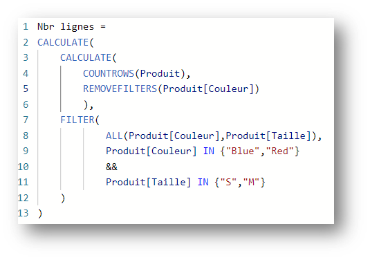
Let’s take another example, with a filter expression on the Color and Size fields:
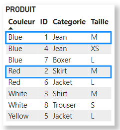
This expression returns 2, i.e. the following 2 lines:
Once again, we have a filter involving 2 columns from the same table. This ” clustering ” principle is applied again, and the FILTER returns a table containing the combinations of distinct values of the columns Product[Color] and Product[Size] according to the filter applied.
Here, the clusters are: {Blue,M},{Red,M}.
The value “S” is not returned, as there is no row of data {Blue,S} or {Red,S}. This is the notion of auto-exist: when creating its clsuters, Power BI returns only those combinations of data actually present in the target table.
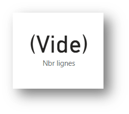
So the following expression doesn’t give 4 as you might expect (the 4 lines with either ” M” or ” S “), but 3 :
Any DAX function that returns a table introduces clusters of values based on the notion of self-existence.
This behavior is the same when the filter system is induced by visuals, via the SUMMARIZECOLUMNS function, which will create clusters when the filtered columns come from one and the same table. Let’s take the following measurement this time:
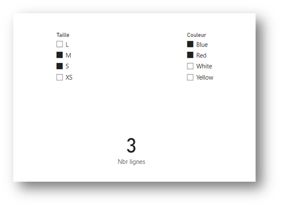
If we configure the same filters on the Color and Size columns, we will obtain exactly the same result, instead of the 4 rows expected for sizes “M” and “S”:
To take the analysis a step further, when a cluster is introduced with a column system and the values of one of these columns are subsequently replaced by another expression, they are replaced within the previously introduced cluster.
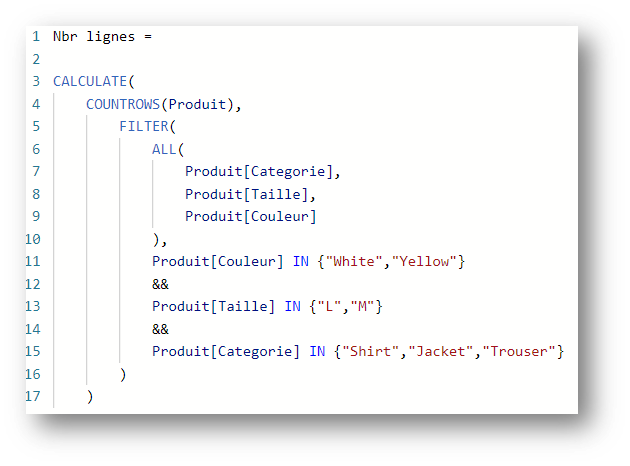
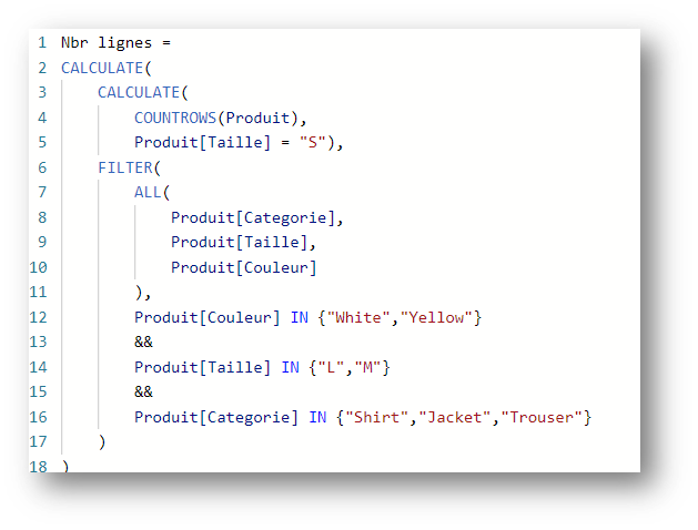
Consider the following measurement:
The following cluster of values is entered in the Categorie, Size and Color columns:
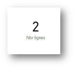
{Jacket,L,Yellow}, {Shirt,M,White}. The measure therefore returns 2.
Let’s make a small modification to the calculation:
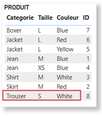
By applying the filter Product[Size] = S in the calculation later, we can expect to replace the previous cluster with the following cluster: {Trouser,S,White}
This is not the case. Because only the Product[Size] field is affected by this new filter. Power BI will transform the filters applied as follows: {Jacket,L,Yellow}, {Shirt,M,White} to ({Jacket,Yellow}, {Shirt,White}) &&. {S}
Instead of returning the {Trouser,S,White} line, this measurement returns an (empty), as there is no corresponding line.
In conclusion, when a DAX function returns a table, or when several fields from the same table are filtered, Power BI introduces a cluster of values for the filtered columns, containing the combinations of distinct values present in the table.
When evaluating a visual, Power BI systematically introduces a SUMMARIZECOLUMNS function.
Auto-exist is then applied to columns from a single table, in the same way as with a table called as a filter argument to a CALCULATE or CALCULATETABLE.
This notion of auto-exist improves processing speed, but can lead to erroneous results when using context functions such as REMOVEFILTER().
This is one of the reasons why star modeling on Power BI is so important.